Hyperbolic Recurrent State-Space Model (H-RSSM)

Project Overview

World models for RL learn a latent representation of the environment and reason entirely within it. In practice, that latent space is almost always Euclidean—which works fine, but isn’t optimal for everything. When you’re dealing with hierarchical structure (trees, nested sub-goals, part-whole relationships), hyperbolic geometry is theoretically superior: it can embed trees with bounded distortion in constant dimension, whereas Euclidean space simply can’t. The problem is computational. The natural distribution on $\mathbb{H}^d$ lacks a closed-form normalising constant, which makes the KL term in the ELBO untractable at training speed.

That’s what I set out to fix. I introduce the Horospherical Gaussian ($\mathcal{HG}$): a distribution family over the upper half-space model of hyperbolic space where the normalising constant, KL divergence between pairs, and reparameterised sampler all have closed-form expressions in $O(d)$, matching the cost of a standard Gaussian RSSM. It’s geometrically motivated but not geodesically exact; I characterise the approximation error explicitly.

On a synthetic $B$-ary tree MDP, the $\mathcal{HG}$ prior does produce depth alignment ($|\rho_\tau|\approx 0.27\text{–}0.31$), but it’s modest and the reconstruction MSE stays well above the observation noise floor. The most interesting empirical result is that alignment extends monotonically to depths the model never saw during training ($\rho_\text{ood} = +0.536$). But it doesn’t hold up. Under $3\times$ longer training, the hyperbolic $\rho$ drops from $0.306$ to $0.200$ while the Euclidean baseline stays flat. Every architectural tweak I tried to strengthen the signal—decoupled KL weights, geometry-aware decoder, action-conditioned prior—either collapsed the representation or got absorbed by the reconstruction loss. This write-up documents what worked, what didn’t, and where I’m still uncertain.

Table of Contents

1. Hyperbolic Latent Spaces
2. The Technical Obstacle: Intractable KL Divergences
3. The Horospherical Gaussian
4. Experimental Setup
5. Results
   • Group A — Baseline claim: does HG induce depth alignment?
     • Experiment 1: τ Spontaneously Encodes Depth
     • Experiment 2: Reconstruction vs Representation
     • Experiment 3: Geometric Inductive Bias Across Seeds
   • Group B — Attempts to strengthen the signal (all fail or trade off)
     • Experiment 4: Separate KL Weights β_τ / β_b
     • Experiment 5: Longer Training (50k steps)
     • Experiment 6: Geometry-Aware Decoder
     • Experiment 7: Action-Conditioned Prior
   • Group C — Where hyperbolic geometry pays off
   • Experiment 8: Dimensional Efficiency — $\mathbb{H}^2$ vs $\mathbb{R}^{32}$
   • Experiment 9: OOD Depth Generalisation
6. Discussion
7. Assumptions and Limitations
8. Code and Reproducibility
9. References
10. Appendix: Derivations
    • A.1 Normalising Constant
    • A.2 Closed-Form KL Divergence
    • A.3 Reparameterisation and Gradient Flow
    • A.4 KL Approximation Error
    • A.5 MGF Identity and Drift Term Stability
    • A.6 Coordinate Change from $(x,y)$ to $(\tau,b)$

1. Hyperbolic Latent Spaces

1.1 Why Hyperbolic Geometry?

World models like DreamerV3 or IRIS jointly learn a compact latent representation of the environment and a transition kernel over it. The agent reasons over latent states, not observations. So the geometry of that latent space shapes everything it can represent and predict.

In practice, we always choose Euclidean geometry: $\mathcal{Z} = \mathbb{R}^d$. It’s the default because it’s computationally convenient.

But many environments have hierarchical structure. Think of an agent navigating nested sub-goals in a grid world, manipulating objects with part-whole relationships, or exploring a maze with branches. In all these cases the state space is tree-like. States multiply exponentially with depth. Euclidean space has polynomial volume growth: the volume of a ball of radius $r$ grows as $r^d$. That means you can’t fit exponential node counts without distorting distances badly. You’d need $O(n)$ dimensions to embed a tree of $n$ nodes with acceptable distortion.

Hyperbolic space is different. It has exponential volume growth: a ball of radius $r$ in $\mathbb{H}^d$ has volume $e^{(d-1)r}$, exactly matching tree structure. Sarkar (2011) showed that any tree of $n$ nodes embeds into $\mathbb{H}^2$ with bounded distortion—constant, independent of $n$—in just 2 dimensions. In Euclidean space, you’d need $d = \Omega(\log n)$.

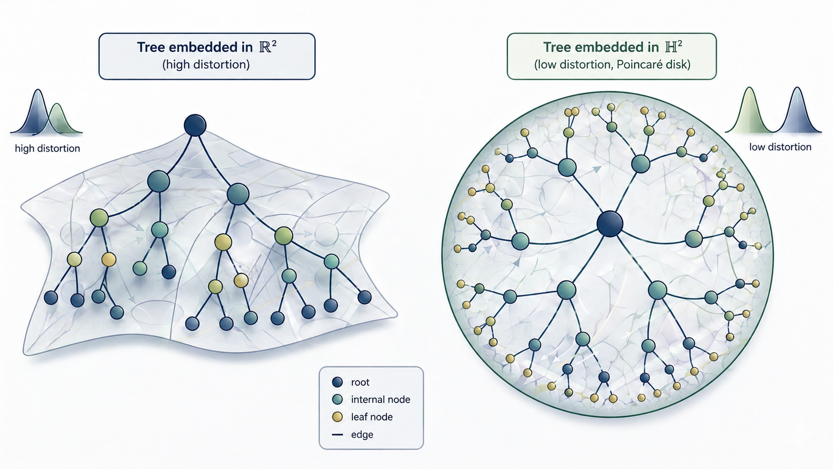
Trees embed efficiently in hyperbolic space ($\mathbb{H}^2$) with bounded distortion, compared to polynomial distortion in Euclidean space ($\mathbb{R}^2$).

1.2 Embedding in $\mathbb{H}^d$

Early work on hyperbolic geometry in ML focused on static embeddings: you have a dataset with known hierarchical structure (a taxonomy, knowledge graph, phylogeny), and you learn to map nodes to $\mathbb{H}^2$ while preserving distances. Nickel & Kiela’s Poincaré embeddings are the classic example. They showed that WordNet hierarchies embed in $\mathbb{H}^2$ with far less distortion than any Euclidean baseline at the same dimension.

The insight is elegant. The Poincaré ball model $\mathbb{B}^d = \{x \in \mathbb{R}^d : \|x\| < 1\}$ with metric $ds^2 = \frac{4\|dx\|^2}{(1-\|x\|^2)^2}$ naturally places the root near the origin (where space is sparse) and leaves near the boundary (where space is exponentially dense). Depth in the hierarchy maps directly to distance from the center.

Poincaré disk with a small tree embedded. Root at center, leaves near boundary

But that’s learning from ground truth. In a world model, you don’t know the structure ahead of time. You have to infer it from observations alone. The embedding becomes a posterior $q_\phi(z_t \mid h_t, o_t)$: a distribution over $\mathbb{H}^d$ that changes at each timestep, learned end-to-end from raw data.

1.3 Learning a Model Inside $\mathbb{H}^d$

That’s where the problems start. Moving from offline static embeddings to a learned generative model introduces three tight constraints, all rooted in the same issue: there’s no tractable Gaussian-like distribution on $\mathbb{H}^d$. Specifically:

• (i) no standard family has a closed-form density with respect to the Riemannian volume
• (ii) without that, the KL in the ELBO has to be estimated by Monte Carlo
• (iii) the reparameterisation trick doesn’t carry over from $\mathbb{R}^d$

Distributions on $\mathbb{H}^d$. A VAE-style world model needs a prior $p_\theta(z_t \mid h_t)$ and a posterior $q_\phi(z_t \mid h_t, o_t)$, both on $\mathbb{H}^d$. The natural choice is the Riemannian Normal $\mathcal{N}_\mathbb{H}(\mu, \sigma^2) \propto e^{-d_\mathbb{H}^2(z, \mu)/2\sigma^2}$, but it has no closed-form normalising constant for $d \geq 2$. Other proposals exist: wrapped normals (Nagano et al., 2019) are computationally heavy; pseudo-hyperbolic Gaussians sacrifice geometric fidelity. None of them are simultaneously tractable, geometrically sound, and fast enough for RL training.

KL divergences. Training requires computing $\mathrm{KL}[q_\phi \| p_\theta]$ at every gradient step. Without a closed form, you resort to Monte Carlo estimation, which kills throughput when you need fast ELBO evaluations. This is why hyperbolic world models haven’t really taken off.

Reparameterisation. You need to backprop through $z \sim q_\phi(\cdot \mid h_t, o_t)$. On a Riemannian manifold, the standard Euclidean reparameterisation trick doesn’t apply directly. Exponential-map approaches exist but blow up numerically near the boundary of the Poincaré ball.

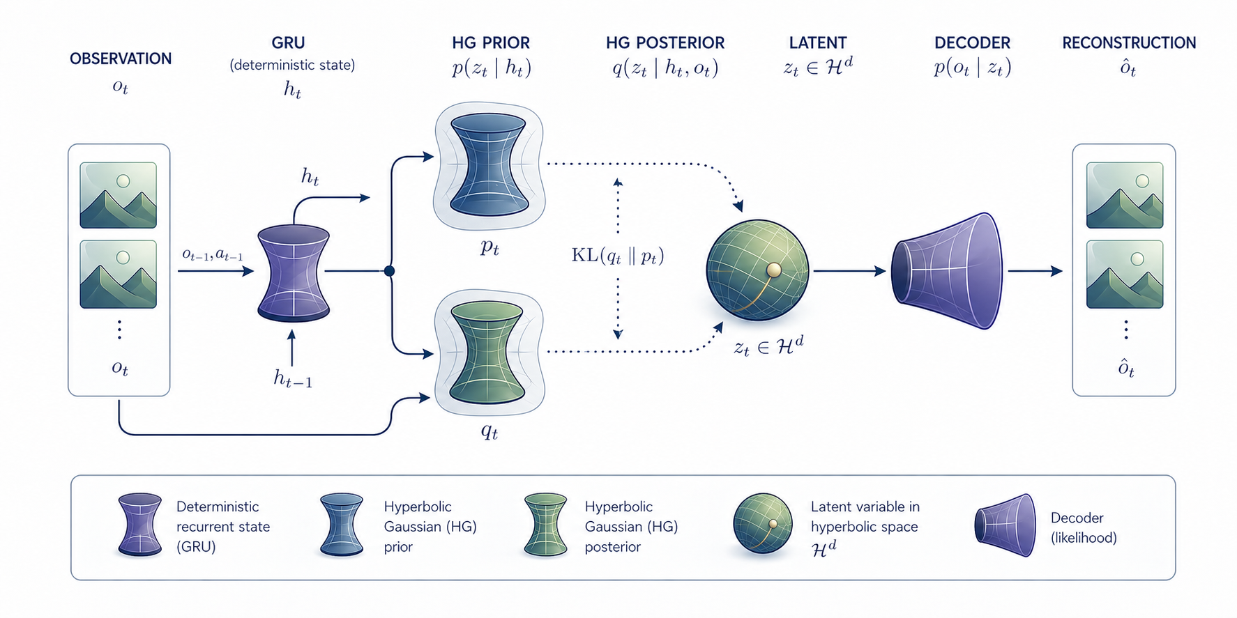
Full model pipeline

My approach solves all three by using the upper half-space model and introducing a new distribution: the Horospherical Gaussian. It’s designed so the KL is exactly tractable in $O(d)$, sampling is exact, and the geometry holds to leading order.

2. The Technical Obstacle: Intractable KL Divergences

World models are trained by maximising the ELBO:

In the Euclidean case both prior and posterior are Gaussian and the KL has a closed form in $O(d)$. On $\mathbb{H}^d$ the natural candidate is the Riemannian Normal, but its normalising constant is the integral that blocks the whole approach:

For every $d \geq 2$ this integral has no closed form. KLs between Riemannian Normals therefore require Monte Carlo estimation, which is far too slow for the per-step ELBO evaluations we need during training. A like-for-like MC estimator would demand a large sample budget per step compared with the $O(d)$ arithmetic of the closed-form alternative I develop below.

This is the problem I set out to fix first.

3. The Horospherical Gaussian

3.1 Construction

I work in the upper half-space model of hyperbolic space, using horospherical (log-height) coordinates:

The metric is

and the Riemannian volume form is

This is the same geometry as the usual upper half-space coordinates $(x,y)$ with $y>0$ after the change of variables $b=x$, $\tau=\log y$ (see A.6 for the derivation). The coordinate $\tau$ is the Busemann coordinate (signed distance to the ideal boundary $\partial\mathbb{H}^d$) and $b$ is the fibre coordinate (the lateral position within a level set). I prefer this model to the Poincaré ball because additive updates $(\tau, b) \leftarrow (\tau + \delta\tau, b + \delta b)$ are globally well-defined and avoid the boundary singularities that can destabilise Möbius-based implementations.

The conditional variance $\mathrm{Var}(b \mid \tau) = e^{2\tau}\sigma_b^2$ is the unique scaling under which the two cancellations below occur.

3.2 Tractability: the two cancellations

Two elementary cancellations are what make the family tractable.

Cancellation 1 (normalising constant). If you integrate out the $b$-component at fixed $\tau$ you pick up a factor $e^{(d-1)\tau}$ that exactly cancels the $e^{-(d-1)\tau}$ in the volume form. The normalising constant evaluates to

independent of $\mu_\tau$ and $\mu_b$ (full derivation in A.1).

Cancellation 2 (drift moment). The tower property gives

Both cancellations are exact and together they make the closed-form KL possible.

Closed-form KL. Combining the cancellations yields a closed-form KL between two $\mathcal{HG}$ distributions (derivation in A.2):

All three terms are exact and total computation is $O(d)$. The drift term follows from the MGF identity $\mathbb{E}[e^{-2\tau}] = e^{-2\mu_\tau^q + 2(\sigma_\tau^q)^2}$. I validated the full expression against a large-sample GPU Monte Carlo estimate: relative error 0.005%.

Reparameterisation. Sampling is exact and straightforward to implement:

Note the coupling of $b$ to $\tau$ through the factor $e^\tau$: it is exact and must be preserved in autograd (see A.3).

3.3 Cost of tractability: $\mathcal{HG}$ is not the Riemannian Normal

The $\mathcal{HG}$ is a tractable approximation rather than the geodesically exact Riemannian Normal. The leading-order discrepancy (see A.4) is

For $d = 16$ and $\sigma = 0.3$ this term evaluates to approximately $2.87$. Whether this approximation error matters in practice is one of the empirical questions the experiments address.

The trade-off summarised:

4. Experimental Setup

4.1 Hypotheses under test

I’m testing three concrete claims, in order:

• H1 (alignment). Training on the ELBO alone is enough for $\mathcal{HG}$ to align its Busemann coordinate $\tau$ with ground-truth depth.
• H2 (capacity). $\mathcal{HG}$ reaches a given level of depth alignment at lower dimension than a Euclidean Gaussian (a sample-efficiency consequence of Sarkar’s theorem).
• H3 (extrapolation). The alignment creates an ordering that extends monotonically to depths never seen in training.

4.2 Environment

I use a $B$-ary tree MDP: a rooted tree with branching factor $B$ and depth $L$. Each node $v$ has a known depth $\ell(v) \in \{0, \ldots, L\}$ and a fixed observation generated by mixing random depth and branch embeddings:

The embeddings $e_v^{\mathrm{depth}}$ and $e_v^{\mathrm{branch}}$ are not given to the model. It only sees $o_v \in \mathbb{R}^{64}$ and has to infer the structure from sequential transitions alone. For the main experiments I use $B = 4$, $L = 5$, which gives 1365 nodes. That suggests a crossover around $d \approx \log_2(1365) \approx 10.4$: below that scale you would expect a Euclidean model to start losing its advantage and struggle with the tree hierarchy relative to $\mathbb{H}^2$.

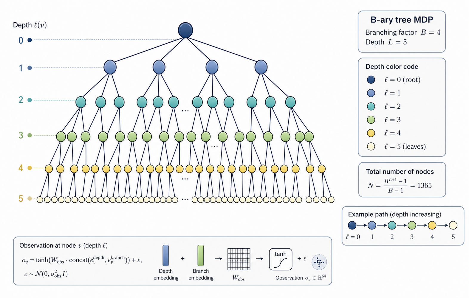
B-ary tree MDP

The observation noise creates a reconstruction MSE floor: if the decoder perfectly reconstructed the clean mean, the residual error from noise alone would be $\mathbb{E}\|\varepsilon\|^2/\dim(o) = \sigma_{\mathrm{obs}}^2$. In my code, $\sigma_{\mathrm{obs}} = 0.05$, which means the per-dimension floor is $\sigma_{\mathrm{obs}}^2 = 0.0025$. I use this later to interpret whether my model’s reconstruction is actually learning anything or just hitting the noise floor.

4.3 Model

I build a sequential world model with GRU recurrence. The prior and posterior are either $\mathcal{HG}$ distributions on $\mathbb{H}^{d}$ (the hyperbolic model) or Gaussians on $\mathbb{R}^{d}$ (the Euclidean baseline). Everything else is held equal: same dimensions, same decoder architecture, same parameter count. This makes the comparison fair: $\mathbb{H}^{d}$ vs $\mathbb{R}^{d}$.

I don’t run any existing hyperbolic-VAE baselines (wrapped normal, Poincaré VAE). This is a real gap (see §7), so the main comparisons in this work are just $\mathcal{HG}$ vs Euclidean Gaussian.

The $\mathcal{HG}$ code path is the same order of complexity as the Euclidean baseline, but I haven’t included a wall-clock benchmark to prove it. That’s something I should add.

4.4 Metrics

I measure four things:

• Reconstruction MSE on held-out test trajectories - interpreted relative to the $\sigma_{\mathrm{obs}}^2 = 0.0025$ floor above.
• Spearman $\rho_\tau$ — correlation between $\mu_\tau^q$ and ground-truth depth (hyperbolic only).
• Linear probes — logistic regression from $\tau$ alone to depth, and from $b$ alone to branch index at depth 1, separating representation quality from reconstruction quality.
• Gradient attenuation $\mathbb{E}[e^{\tau_t}]$ - measuring the amplification of $b$-gradients through the reparameterisation coupling.

4.5 Reporting convention

Except where I explicitly say otherwise, every table below shows a single training run per configuration. Computing limits meant I couldn’t afford many seeds. The only multi-seed estimate is Experiment 3 (5 seeds), which gives me a variance band of roughly $\pm 0.05$ in $\rho$. If you see a difference in $\rho$ smaller than 0.05 between two runs, it’s probably within that noise band and shouldn’t be trusted as a real effect.

5. Results

I’ve grouped the experiments into three blocks:

• (A) the baseline claim that $\mathcal{HG}$ induces depth alignment
• (B) four attempts to strengthen that signal, each one either trading off against MSE or collapsing the prior
• (C) the two findings where hyperbolic geometry does provide something Euclidean does not: dimensional efficiency and out-of-distribution depth ordering

Group A - Baseline claim: does HG induce depth alignment?

Experiment 1: τ Spontaneously Encodes Depth

Question. Trained purely on the ELBO with no depth supervision, does the Busemann coordinate $\tau$ end up correlated with ground-truth depth?

Setup. Single seed, $d = 16$, standard $\mathcal{HG}$ prior/posterior.

Result. The hyperbolic model achieves $\rho_\tau \approx +0.306$ on a single run. The Euclidean baseline achieves $\rho_\mathrm{pc1} = 0.275$ at $d = 16$ (best principal component, the strongest possible PCA baseline). The difference is small and must be read together with Exp 3, which quantifies seed variance at $\pm 0.05$. $\tau$ also shows a positive correlation with depth without supervision. Whether this constitutes a robust “advantage” over the Euclidean baseline is a question Exp 3 addresses directly.

The drift term penalises fibre mismatch less when $\tau$ is larger. So if deeper nodes usually have more fibre mismatch, the model is pushed toward larger $\tau$ for those nodes. This depth-to-fibre-mismatch link is only a hypothesis here; we did not measure it directly.

Experiment 2: Reconstruction vs Representation

Question. Do hyperbolic latent dimensions improve either reconstruction or representation quality?

Setup. Sweep $d \in \{2, 4, 8, 16, 32\}$, 15 000 training steps, KL warmup, single seed.

Reconstruction (MSE). Both models stay at $\approx 0.405$ across every dimension, differing by $< 0.001$. With $\sigma_{\mathrm{obs}}^2 = 0.0025$, these are far above the noise floor, so what I’m comparing here is model reconstruction quality, not noise saturation.

Representation. $|\rho_\tau|$ ranges 0.266–0.321 across $d$, essentially flat within seed noise. The $\tau \to$ depth probe sits flat at 0.68 across all dimensions. This could mean one of two things:

• (i) the depth signal in $\tau$ genuinely caps at the probe’s capacity,
• (ii) or the logistic-regression probe is saturated by the tree’s depth class imbalance. My current data doesn’t distinguish between them.

The $b \to$ branch probe never converges. Experiment 4 revises my interpretation: it’s a regularisation artefact, not a structural property of the fibre coordinate.

Reconstruction MSE vs dimension. Euclidean (orange) stays flat; hyperbolic (blue) moves within a negligible range. Both remain far above the observation-noise floor.

Linear probe accuracy. Blue circles: depth from $\tau$ at 0.68, flat across $d$. The $b \to$ branch probe did not converge.

Experiment 3: Geometric Inductive Bias Across Seeds

Question. Is that modest hyperbolic advantage in Exp 1 larger than seed noise, or is it just a fluke?

Setup. Both models at $d = 16$, 2000 steps, 5 seeds each. Computing limits kept me from running more. I logged Spearman $\rho$ between $\mu_\tau^q$ and depth every 100 steps (hyperbolic), and best-PCA $|\rho|$ across all components for Euclidean (the strongest possible baseline). Shaded regions show ±1σ across seeds.

Mean $\rho$ at step 2000: hyperbolic $0.277 \pm 0.052$, Euclidean $0.271 \pm 0.054$. The two are indistinguishable in both mean and variance. The Euclidean model starts with high accidental alignment (best-PC cherry-picked from random init), then settles to the same regime as hyperbolic. The hyperbolic trajectory starts lower but rises from step 0.

Within the noise from this experiment, hyperbolic and Euclidean reach the same depth-alignment magnitude at step 2000. What differs is the trajectory, not where they end up. So the honest headline for the depth-alignment claim is: Exp 1’s single-seed $0.306$ vs $0.275$ sits right within the $\pm 0.05$ noise band.

What this does not show. I report absolute values of $\rho$, which hides the sign. A geometric inductive bias is only as strong as the sign consistency across seeds. Without checking the sign across all five seeds, I can’t verify the “consistent push toward deeper = higher $\tau$” story directly, even though the mechanism supports it.

The drift term $\frac{\|\mu_b^q - \mu_b^p\|^2}{2(\sigma_b^p)^2} \cdot e^{-2\mu_\tau^q + 2(\sigma_\tau^q)^2}$ penalises fibre mismatch in proportion to $e^{-2\mu_\tau^q}$, which creates a directional gradient pushing larger $\tau$ for nodes that diverge from the prior. But the signal-to-noise threshold for reconstructing tree-like structure (Kesten–Stigum, 1966) is not met at $B=4$, so the maximum attainable $\rho$ stays capped regardless of geometry.

Group B - Attempts to strengthen the signal (all fail or trade off)

Below I try four different architectural levers to amplify the depth-encoding bias. Each one fails or introduces a matching cost elsewhere.

Experiment 4: Separate KL Weights β_τ / β_b

Question. In Experiments 1–3 I used a single $\beta$ to weight all KL terms equally. But the fibre KL is weighted by $(d-1)$ and dominates the height KL at large $d$. What if I decouple the weights ($\beta_\tau$ for the height term, $\beta_b$ for the fibre and drift terms) to improve the depth signal without hurting reconstruction?

Setup. Single seed, $d=16$, sweep over $\beta_\tau$ and $\beta_b$.

Reducing $\beta_b$ reveals a sharp trade-off. At $\beta_b = 0.1$, MSE drops 11% (0.405 → 0.363) with only marginal loss in $\rho$: a clear MSE vs depth trade, but still far above the noise floor. At $\beta_b = 0.01$, MSE collapses to 0.068 but $\rho_\tau$ collapses to 0.016: the model stops encoding depth and just learns a trivial reconstruction. Doubling $\beta_\tau$ to 2.0 with $\beta_b = 0.1$ doesn’t recover the depth signal ($\rho = 0.304$).

What this reveals about Exp 2’s $b \to$ branch null. The $b$-probe never converged in Exp 2. Here I see that the fibre KL wasn’t suppressing $b$ in a way that encoded branch structure elsewhere: it was just acting as a regulariser that prevents MSE collapse. Remove it and MSE drops but the latent becomes unstructured. So I should revise my original reading of the branch-probe failure from “structural constraint” to “regularisation artefact”.

What this does not show. The $\beta_b=0.1$ MSE drop is tempting, but $\rho$ moves the wrong way. The trade-off is real; the best setting is just the unweighted default.

Experiment 5: Longer Training (50k steps)

Question. Does the depth alignment from Exp 1–3 strengthen with more training, stabilise, or erode?

Setup. $d=16$, 50 000 steps (3× longer than Exp 2), single seed, direct comparison to the 15k numbers.

MSE doesn’t move for either model. The hyperbolic $\rho$ erodes from 0.306 to 0.200, falling below the Euclidean baseline at 0.276. This erosion is specific to HG, it’s not a generic over-training effect.

The drift term creates a depth-aligning gradient early in training, but the (Euclidean) MSE reconstruction objective doesn’t reinforce it. As optimisation continues, $\mu_\tau^q$ drifts toward whatever value minimises reconstruction, which isn’t necessarily depth-correlated. The Euclidean model, lacking any geometric inductive bias to lose, settles into a stable local minimum.

This same erosion mechanism (geometric structure in the prior being absorbed by reconstruction pressure) shows up again as an explicit parameter collapse in Exp 7.

What this does not show. Single seed; I don’t know the magnitude of erosion across different seeds.

Experiment 6: Geometry-Aware Decoder

Question. The decoder in all previous experiments receives $(\tau, b)$ as a flat vector and is not told that $\tau$ is a Busemann coordinate. If I give the decoder explicit geometric features, does that improve reconstruction or representation?

Setup. Augment the decoder input with $e^\tau$ (metric scaling factor) and $\|b\|^2 e^{-2\tau}$ (squared $b$-distance in the hyperbolic metric). Single seed, $d=16$.

The geometry-aware decoder does not help. It slightly worsens both $\rho_\tau$ (+0.270 vs +0.295) and the depth probe (0.632 vs 0.680), and it does so with no MSE improvement.

I think this is a classic representation-collapse dynamic. Exposing $e^\tau$ and $\|b\|^2 e^{-2\tau}$ directly gives the decoder a reconstruction shortcut that removes the encoder’s incentive to encode depth cleanly in $\tau$. The pressure that created the structured representation is gone, and the MSE stays unchanged because both paths reach essentially the same reconstruction level.

Future work. Gating or annealing the shortcut features, for example warm-starting with flat input and slowly exposing the geometric features, might preserve the encoder pressure. I have not tested that.

Experiment 7: Action-Conditioned Prior

Question. Exp 5 showed depth alignment erodes under extended training. Can injecting action labels directly into the prior make depth alignment an explicit structural objective rather than a fragile KL side effect?

Setup. Augment the prior with an action-conditioned offset to $\mu_\tau^p$:

where $a_{t-1} \in \{-1, 0, +1\}$ encodes the direction of the last transition (deeper / shallower / same level) and $\alpha, \beta$ are learned scalars.

At step 5k the action prior reaches $\rho = 0.755$, which is an exceptional early alignment and far above the standard model’s $\rho = 0.080$. That advantage disappears by step 15k, and both models converge to $\rho \approx 0.27$ by step 30k. The learned bias parameters collapse to near zero: $\text{softplus}(\alpha) = 0.0008$, $\text{softplus}(\beta) = 0.0008$. In practice, the model learns to ignore its own structural prior.

The action prior functions as a warm-start mechanism, not a stable structural constraint. Early in training the action signal provides a strong depth gradient that initialises $\tau$ well. As optimisation continues, the reconstruction loss dominates and the model adapts by zeroing out the prior bias, which is the same failure mode as Exp 5 but reached faster and more visibly.

What this does not show. I have not tested whether a non-learnable action offset, with frozen $\alpha$ and $\beta$, would preserve the early alignment.

Group C - Where hyperbolic geometry pays off

Experiment 8: Dimensional Efficiency - $\mathbb{H}^2$ vs $\mathbb{R}^{32}$

Question. Sarkar (2011) proves any finite tree embeds into $\mathbb{H}^2$ with distortion converging to 1. In the learning setting, can a 2-dimensional hyperbolic latent capture depth as well as a 32-dimensional Euclidean latent?

Setup. Train each model at $d \in \{2, 4, 8, 16, 32, 64\}$ (where defined), 15k steps, single seed per cell.

Three things are true here, and only one of them is what Sarkar predicts:

1. $\mathbb{H}^2$ matches $\mathbb{R}^{32}$ within noise (0.264 vs 0.277). Consistent with the capacity advantage.
2. Neither model benefits from dimension. Hyperbolic $|\rho_\tau|$ is flat at 0.26–0.28 across $d = 2\ldots 32$; Euclidean $|\rho|$ is similarly flat at 0.26–0.28 across $d = 4\ldots 32$. Sarkar predicts the hyperbolic model should beat Euclidean at matched low $d$ — that is not observed.
3. $\mathbb{R}^{64}$ collapses to 0.071. This is almost certainly an optimisation artefact (best-PC drift at high $d$ with a fixed training budget), not a capacity failure.

The honest reading is therefore: H² is not worse than R³² on this metric, and neither model is capacity-limited in the tested range. This is consistent with Sarkar’s theorem carrying over to the learning setting but does not cleanly demonstrate the predicted advantage, because both models are in a regime where added dimensions are not helping.

The flatness in $|\rho_\tau|$ is a separate, interpretable finding: all depth information in $\mathcal{HG}$ is carried by the scalar $\tau$ by construction; the fibre coordinates $b \in \mathbb{R}^{d-1}$ are depth-uninformative by design. Adding fibre dimensions cannot change $\rho_\tau$.

What this does not show. A clean dimensional-efficiency advantage would require a setting where Euclidean $\rho$ grows with $d$, so that the capacity curve is visible, while hyperbolic saturates at low $d$. At the observation-noise and training-budget levels here, no such curve appears.

Experiment 9: OOD Depth Generalisation

Question. Does the depth ordering induced by $\mathcal{HG}$ extend to depths the model never saw in training?

Setup. Train on a deeper tree ($B=4$, $L=7$) with walks restricted to depth $\leq 5$. Evaluate $\rho_\tau$ separately on in-distribution nodes (depth 0–5) and OOD nodes (depth 6–7). Compare the standard $\mathcal{HG}$ to the ActionPrior variant from Exp 7.

Caveat, stated up front. The OOD depth range covers 2 levels (6, 7) versus 6 levels (0..5) in-distribution. A scalar correlation over a 2-level range is simpler than over a 6-level range and tends to give larger magnitudes. The sign and consistency of the OOD ranking are the load-bearing claims; the magnitude comparison to in-distribution $\rho$ is not.

The standard $\mathcal{HG}$ model achieves $\rho_\text{ood} = +0.536$. The sign is correct, the magnitude is strong, and the model has never seen depth 6 or 7 in training. The induced ordering, deeper to higher $\tau$, extends monotonically beyond the training range. This is the hardest result to explain without the hyperbolic geometry, because the drift term’s penalty structure creates a ranking that comes from the KL objective rather than memorised depth values.

The ActionPrior variant inverts the OOD ordering ($\rho_\text{ood} = -0.511$). This is not a small degradation, because the model actively predicts that deeper nodes are shallower. Combined with Exp 7’s bias-parameter collapse ($\text{softplus}(\alpha) = 0.0008$), this suggests the ActionPrior creates a subtly distorted geometry that does not extrapolate. Structural priors that learn to zero out their own parameters can break the geometry they were meant to reinforce.

What this does not show. This is still single-seed. I have not tested whether the OOD result holds across seeds, and given Exp 3’s seed variance on in-distribution $\rho$, a multi-seed replication of Exp 9 is the single most important follow-up. I also have not tested whether OOD generalisation degrades with extended training in the same way as in-distribution $\rho$ did in Exp 5.

6. Discussion

The strongest result in this work is Experiment 9: the standard $\mathcal{HG}$ model induces a depth ordering that extends monotonically to depths it never saw during training ($\rho_\text{ood} = +0.536$), while the ActionPrior variant, whose learned bias collapses to $\approx 0.0008$, inverts that ordering ($\rho_\text{ood} = -0.511$). The positive case is the clearest sign that the geometry is acting like a structural property of the objective rather than a memorised fit to the training set. I still need to keep the caveat from Exp 9 in mind: the OOD $\rho$ is computed over a 2-level depth range, so it should not be read as absolute evidence that the model is “generally better” at extrapolation.

The rest of the picture is more mixed. I summarise the evidence as honestly as I can:

What works. The $\mathcal{HG}$ construction itself, namely closed-form KL at $O(d)$, exact reparameterisation, no Möbius singularities, and a controlled approximation error, is the load-bearing contribution. The OOD result in Exp 9 is the sharpest empirical sign that the geometry is doing something the Euclidean baseline cannot do.

What doesn’t work. Every architectural lever I tried to strengthen the in-distribution depth signal either created a trade-off (Exp 4: MSE versus $\rho$), introduced a shortcut (Exp 6: representation collapse), or got absorbed by the reconstruction loss (Exp 5, Exp 7). My reading of that pattern is simple: Euclidean reconstruction pressure erodes hyperbolic structure because good reconstruction does not require good geometric alignment.

A speculative path forward, not evidence. Replacing Euclidean MSE with a geodesic reconstruction loss on $\mathbb{H}^d$ would couple reconstruction directly to the hyperbolic metric and might make geometric alignment a prerequisite for low loss rather than a side effect. That is a hypothesis, not a result.

7. Assumptions and Limitations

Taken in rough order of how much each point matters:

Single-seed main tables. Experiments 1, 2, 4, 5, 6, 7, 8, 9 report single training runs. Exp 3 (5 seeds, $\pm 0.052$) is the only variance estimate, and it shows that the single-seed $\rho$ differences of $< 0.05$ elsewhere are within seed noise. The OOD result ($\rho_\text{ood} = +0.536$) especially needs multi-seed replication before I would cite it confidently.

MSE floor $\approx \sigma_\mathrm{obs}^2$. The observation noise $\sigma_\mathrm{obs}$ in the tree MDP is 0.05, so the per-dimension floor is $\sigma_\mathrm{obs}^2 = 0.0025$. The recurring value 0.405 across Exps 2, 5, 6 is far above this floor, so cross-model MSE comparisons are informative here.

Unverified mechanism. The drift-term explanation for why $\tau$ aligns with depth requires that deeper nodes have higher fibre mismatch on average. That is plausible for typical random-walk trajectories on the tree, but I did not measure it directly.

No hyperbolic-VAE baseline. The baseline comparison is $\mathcal{HG}$ versus Euclidean Gaussian only. Existing hyperbolic alternatives, such as wrapped normals (Nagano et al., 2019) and Poincaré VAEs (Mathieu et al., 2019), were not run. Claims of “computational parity” are against Euclidean only, and the representation-quality results do not show that $\mathcal{HG}$ beats other hyperbolic distributions.

$\mathcal{HG}$ approximation error. $\mathrm{KL}[\mathcal{N}_\mathbb{H}\|\mathcal{HG}] = \frac{d^2-1}{8}\sigma^2 + O(\sigma^3)$. For $d \geq 8$ and typical posterior widths this is not small, so the optimisation target is not geodesically correct.

Sign of $\rho_\tau$. Exp 3 reports $|\rho|$, not $\rho$. Cross-seed sign consistency, which is crucial for the “geometric inductive bias” claim, is inferred from the drift-term mechanism but not measured.

GRU architecture. The GRU treats $(\tau_{t-1}, b_{t-1})$ as a flat Euclidean vector, with no inductive bias toward using $\tau$ for depth or $b$ for branch. An architecture with attention over hyperbolic representations, or a genuine hyperbolic recurrence, might produce qualitatively different results.

Synthetic, fully-balanced tree. The tree MDP is maximally hierarchical. Real environments have weaker, irregular, and potentially non-tree-like structure. Whether $\mathcal{HG}$ helps there is untested.

Compute parity is claimed, not measured.

8. Code and Reproducibility

All experiments are implemented in PyTorch. The hrssm library contains the $\mathcal{HG}$ distribution with closed-form KL (validated against Monte Carlo, relative error 0.005%), the $B$-ary tree MDP with OOD depth support, and all world model variants. Experiments 1–6 run in h_rssm_gpu.ipynb; Experiments 7–9 run in experiments_v2.ipynb, both Kaggle-compatible.

The three formulas needed to reproduce the key results:

• KL: $\mathrm{KL}[q\|p] = \text{height KL} + (d-1) \cdot \text{fibre KL} + \text{drift term}$, as given above.
• Reparameterisation: $\tau = \mu_\tau^q + \sigma_\tau^q \varepsilon_1$, $b = \mu_b^q + e^\tau \sigma_b^q \varepsilon_2$ (coupling must be preserved).
• Gradient attenuation diagnostic: $\mathbb{E}[e^{\tau_t}] = e^{\mu_\tau^q + (\sigma_\tau^q)^2/2}$.

9. References

• Ganea, O., Bécigneul, G., & Hofmann, T. (2018). Hyperbolic neural networks. NeurIPS.
• Gu, A., Sala, F., Gunel, B., & Ré, C. (2019). Learning mixed-curvature representations in product spaces. ICLR.
• Hafner, D. et al. (2019). Learning latent dynamics for planning from pixels (PlaNet). ICML.
• Hafner, D. et al. (2023). Mastering diverse domains with world models (DreamerV3). arXiv:2301.04104.
• Mathieu, E. et al. (2019). Continuous hierarchical representations with Poincaré variational auto-encoders. NeurIPS.
• Micheli, V., Alonso, E., & Fleuret, F. (2022). Transformers are sample-efficient world models (IRIS). ICLR 2023.
• Nagano, Y. et al. (2019). A wrapped normal distribution on hyperbolic space for gradient-based learning. ICML.
• Nickel, M., & Kiela, D. (2017). Poincaré embeddings for learning hierarchical representations. NeurIPS.
• Sarkar, R. (2011). Low distortion Delaunay embedding of trees in hyperbolic plane. Graph Drawing.

Appendix: Derivations

A.1 Normalising Constant of the Horospherical Gaussian

The unnormalised density w.r.t. the Riemannian volume form $d\mathrm{vol} = e^{-(d-1)\tau}\,d\tau\,db$ is:

Step 1 (integrate over $b$ at fixed $\tau$).

This is a $(d-1)$-dimensional Gaussian integral with variance $e^{2\tau}\sigma_b^2$ per dimension:

Step 2 (the key cancellation). The volume form contributes $e^{-(d-1)\tau}$. Multiplying:

The $\tau$-dependence of the $b$-integral cancels exactly against the volume form. The remaining integral is purely over $\tau$:

This is independent of $\mu_\tau$ and $\mu_b$, which is exactly what I need for closed-form KL divergences.

A.2 Closed-Form KL Divergence

Let $q = \mathcal{HG}(\mu_\tau^q, \mu_b^q, \sigma_\tau^q, \sigma_b^q)$ and $p = \mathcal{HG}(\mu_\tau^p, \mu_b^p, \sigma_\tau^p, \sigma_b^p)$.

The log-density w.r.t. $d\mathrm{vol}$ is:

The KL divergence is $\mathrm{KL}[q\|p] = \mathbb{E}_q[\log q(\tau,b) - \log p(\tau,b)]$.

Taking the difference of log-densities:

Height KL. Taking $\mathbb{E}_q$ over $\tau$ (which marginally is $\mathcal{N}(\mu_\tau^q, (\sigma_\tau^q)^2)$):

Combined with $\log Z_p/Z_q$ for the $\tau$ part ($\log\sigma_\tau^p/\sigma_\tau^q$):

Fibre terms. Expand $\|b - \mu_b^p\|^2 = \|b - \mu_b^q\|^2 + 2(b-\mu_b^q)^\top(\mu_b^q - \mu_b^p) + \|\mu_b^q - \mu_b^p\|^2$. Taking $\mathbb{E}_q$ conditioned on $\tau$, using $\mathbb{E}[b|\tau] = \mu_b^q$:

Second cancellation and the drift term. Taking $\mathbb{E}_q$ over $\tau$ for the second part:

Since $\tau \sim \mathcal{N}(\mu_\tau^q, (\sigma_\tau^q)^2)$, the moment generating function at $s = -2$ gives:

This is the drift term. Combined with the $\log Z_p/Z_q$ contribution for $b$ (which is $(d-1)\log\sigma_b^p/\sigma_b^q$) and $\mathbb{E}_q[-\|b-\mu_b^q\|^2 / 2e^{2\tau}(\sigma_b^q)^2] = -(d-1)/2$:

Assembling all terms:

All three terms are $O(d)$ to compute.

A.3 Reparameterisation and Gradient Flow

Sampling. Draw $\varepsilon_1 \sim \mathcal{N}(0,1)$ and $\varepsilon_2 \sim \mathcal{N}(0, I_{d-1})$:

Correctness. The marginal of $\tau$ is $\mathcal{N}(\mu_\tau^q, (\sigma_\tau^q)^2)$ by construction. The conditional $b|\tau$ is:

which matches $\mathrm{Var}(b|\tau) = e^{2\tau}(\sigma_b^q)^2$ from the $\mathcal{HG}$ definition. The coupling $b = f(\mu_\tau^q, \sigma_\tau^q, \mu_b^q, \sigma_b^q, \varepsilon_1, \varepsilon_2)$ is fully differentiable.

Gradient attenuation. The gradient of the decoder loss w.r.t. $\mu_b^q$ passes through $\partial b/\partial \mu_b^q = I$, but w.r.t. $\mu_\tau^q$ it passes through $\partial b/\partial \mu_\tau^q = e^\tau \sigma_b^q \varepsilon_2$. The expected magnitude of this gradient amplification factor is:

by the MGF of a Gaussian at $s = +1$. When $\mathbb{E}[e^\tau] \gg 1$, gradients from the fibre reconstruction are amplified into $\mu_\tau^q$ and can destabilise $\tau$ training, which is the gradient attenuation diagnostic reported in Experiment 2.

A.4 KL Approximation Error

The $\mathcal{HG}$ is not the Riemannian Normal $\mathcal{N}_\mathbb{H}(\mu, \sigma^2)$. To quantify the discrepancy, consider the isotropic case $\mu_\tau = 0$, $\mu_b = 0$, $\sigma_\tau = \sigma_b = \sigma$, and compare with $\mathcal{N}_\mathbb{H}(\mathbf{0}, \sigma^2)$ whose density w.r.t. $d\mathrm{vol}$ is proportional to $e^{-d_\mathbb{H}^2(z,\mathbf{0})/2\sigma^2}$.

In the upper half-space, the geodesic distance from the origin $(\tau=0, b=0)$ satisfies:

The $\mathcal{HG}$ density exponent is $-(\tau^2/2\sigma^2 + e^{-2\tau}\|b\|^2/2\sigma^2)$, so it agrees with $\mathcal{N}_\mathbb{H}$ to leading order. The discrepancy arises from higher-order terms in the geodesic distance expansion. A Taylor expansion gives:

The leading coefficient $\frac{d^2-1}{8}$ grows quadratically with $d$. At $d = 16$, $\sigma = 0.3$: error $\approx \frac{255}{8} \times 0.09 \approx 2.87$. I do not think this is negligible for large $d$ or large posterior widths, and I treat it as the main theoretical limitation of $\mathcal{HG}$ as an approximation to the Riemannian Normal.

A.5 MGF Identity and Drift Term Stability

The drift term involves $e^{-2\mu_\tau^q + 2(\sigma_\tau^q)^2}$, which can grow without bound as $\sigma_\tau^q \to \infty$. In practice, a clamp at $\log \text{MGF} \leq 10$ is applied before exponentiation to prevent KL overflow during early training when posteriors are wide.

The full drift is bounded by:

After warmup, posteriors narrow and $\sigma_\tau^q \to 0$, so $e^{-2\mu_\tau^q + 2(\sigma_\tau^q)^2} \to e^{-2\mu_\tau^q}$ and the drift naturally weights fibre mismatch by $e^{-2\mu_\tau^q}$, which penalises shallow nodes more than deep ones. This is the mechanism I rely on when I say that high fibre mismatch pushes $\mu_\tau^q$ upward and produces positive $\rho_\tau$.

A.6 Coordinate Change from $(x,y)$ to $(\tau,b)$

Step 1 (starting model). Start from the standard upper half-space model

with metric and volume form

Step 2 (change of variables). Define

Because $\log : (0,\infty) \to \mathbb{R}$ is a smooth bijection with smooth inverse $\exp$, this is a global diffeomorphism in the vertical coordinate, so $\tau \in \mathbb{R}$ (hence can range from $-\infty$ to $+\infty$).

Step 3 (differentials).

Step 4 (metric substitution). Substitute into $g$:

Step 5 (volume-form substitution). Use the Jacobian determinant of $(\tau,b) \mapsto (y,x) = (e^{\tau}, b)$: